Law of total cumulance
In probability theory and mathematical statistics, the law of total cumulance is a generalization to cumulants of the law of total probability, the law of total expectation, and the law of total variance. It has applications in the analysis of time series. It was introduced by David Brillinger.[1]
It is most transparent when stated in its most general form, for joint cumulants, rather than for cumulants of a specified order for just one random variable. In general, we have
where
- κ(X1, ..., Xn) is the joint cumulant of n random variables X1, ..., Xn, and
- the sum is over all partitions
 of the set { 1, ..., n } of indices, and
- "B ∈ π" means B runs through the whole list of "blocks" of the partition π, and
- κ(Xi : i ∈ B | Y) is a conditional cumulant given the value of the random variable Y. It is therefore a random variable in its own right—a function of the random variable Y.
Contents |
Examples
The special case of just one random variable and n = 2 or 3
Only in case n = either 2 or 3 is the nth cumulant the same as the nth central moment. The case n = 2 is well-known (see law of total variance). Below is the case n = 3. The notation μ3 means the third central moment.
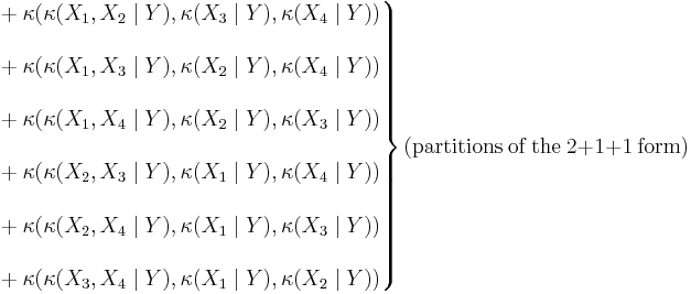
General 4th-order joint cumulants
For general 4th-order cumulants, the rule gives a sum of 15 terms, as follows:
Cumulants of compound Poisson random variables
Suppose Y has a Poisson distribution with expected value 1, and X is the sum of Y independent copies of W.
All of the cumulants of the Poisson distribution are equal to each other, and so in this case are equal to 1. Also recall that if random variables W1, ..., Wm are independent, then the nth cumulant is additive:
We will find the 4th cumulant of X. We have:
-
 (the punch line—see the explanation below).
We recognize this last sum as the sum over all partitions of the set { 1, 2, 3, 4 }, of the product over all blocks of the partition, of cumulants of W of order equal to the size of the block. That is precisely the 4th raw moment of W (see cumulant for a more leisurely discussion of this fact). Hence the moments of W are the cumulants of X.
In this way we see that every moment sequence is also a cumulant sequence (the converse cannot be true, since cumulants of even order ≥ 4 are in some cases negative, and also because the cumulant sequence of the normal distribution is not a moment sequence of any probability distribution).
Conditioning on a Bernoulli random variable
Suppose Y = 1 with probability p and Y = 0 with probability q = 1 − p. Suppose the conditional probability distribution of X given Y is F if Y = 1 and G if Y = 0. Then we have
where  means π is a partition of the set { 1, ..., n } that is finer than the coarsest partition – the sum is over all partitions except that one. For example, if n = 3, then we have
References
- ^ David Brillinger, "The calculation of cumulants via conditioning", Annals of the Institute of Statistical Mathematics, Vol. 21 (1969), pp. 215–218.


